Hello fPocket
Show how to use fPocket to find locations to dock the ligands
fPocket - finds canidate locations to dock the ligand
Step 1: Get back into your lab environment.
Using the terminal, change to the directory with your target protein and activate your biolab conda environment. You may need to change the cd command below depending on your folder structure.
        cd Documents/MolecularBonding/locks/
        conda activate biolab
Step 2: We will be using the same protien from the previous lesson, 1H9Z. Run fPocket on this protein.
fpocket -f 1H9Z.pdb
The output text is underwhelming, the magic is in the files fPocket creates.
        ***** POCKET HUNTING BEGINS *****
        ***** POCKET HUNTING ENDS *****
fPocket has now created a folder called 1H9Z_out. This folder contains the following:
1H9Z_info.text - This file shows all the pocket fPocket has found along with the stats of the pocket.
1H9Z_out.pdb - This is the original protein file with the pocket information, allowing you to color the pocket with PyMol.
1H9Z_pockets.pqr - This contains the alpha spheres, the virtual marbles used to fill the holes.
1H9Z_PYMOL.sh - This is a script. When ran it will open PyMol and load the protein and ligand with some styling.
pockets - This is a folder. The files in this folder contains information about all the pockets it found.
Step 3: Evaluating the output
Open 1H9Z_info.txt with a text editor to view it's contents. Below is the what fPocket found for the first pocket. fPocket will put what it consideres best canidates at the top, IE Pocket 1 is considered a better canidate than Pockket 40.
        Pocket 1 :
            Score : 	2.370
            Druggability Score : 	0.996
            Number of Alpha Spheres : 	617
            Total SASA : 	714.062
            Polar SASA : 	224.280
            Apolar SASA : 	489.782
            Volume : 	4476.194
            Mean local hydrophobic density : 	67.850
            Mean alpha sphere radius :	3.949
            Mean alp. sph. solvent access : 	0.467
            Apolar alpha sphere proportion : 	0.627
            Hydrophobicity score:	35.510
            Volume score: 	 4.388
            Polarity score:	 43
            Charge score :	 11
            Proportion of polar atoms: 	32.698
            Alpha sphere density : 	16.598
            Cent. of mass - Alpha Sphere max dist: 	40.507
            Flexibility : 	0.12
These are the most important stats:
Score - Overall score, higher is usually better
Druggability Score - Scale is 0 - 1. Higher is better, .5 and above is considered "druggable".
Volume - Volume of the cavity/pocket. It must be big enough so the ligand can fit into it.
Hydrophobicity - Higher numbers are often better, because of the hydrophobic effect.
Step 4: Put the data generated by fPocket to use.
We will take the top canidate, Pocket 1, and find it's center. We will then try to dock the ligand to see
how well of a bond it makes. We will then view the results with PyMol.
Switch to the pocket foler and then open pymol:
        cd ~/Documents/MolecularDocking/locks/1H9Z_out/pockets
        plymol
Enter these command into PyMol's terminial
        load pocket1_vert.pqr
        pseudoatom pocket_center, pocket1_vert
        print cmd.get_coords('pocket_center')
You will get some output that looks like this:
        PyMOL>pseudoatom pocket_center, pocket1_vert
        ObjMol: created pocket_center/PSDO/P/PSD`1 /PS1
        PyMOL>print cmd.get_coords('pocket_center')
        [[23.093771  8.962    14.027454]]
Update your config file with the new x, y, z coordinates. My config file is located here:
~/Documents/MolecularDocking/config.txt
        receptor = ./locks/receptor.pdbqt
        ligand = ./keys/warfarin.pdbqt

        center_x = 23.09
        center_y = 8.96
        center_z = 14.03

        size_x = 25.0
        size_y = 25.0
        size_z = 25.0

        thread = 8000
        search_depth = 10

        energy_range = 4
Step 5: Run AutoDock-Vina-GPU-2
~/software/Vina-GPU-2.1/AutoDock-Vina-GPU-2.1/AutoDock-Vina-GPU-2-1 --config config.txt
Here is the output from AutoDock
        #################################################################
        # If you used AutoDockVina-GPU 2.1 in your work, please cite:   #
        #                                                               #
        # Ding, Ji, et al. Vina-GPU 2.0: Further Accelerating AutoDock  #
        # Vina and Its Derivatives with Graphics Processing Units.      #
        # Journal of Chemical Information and Modeling (2023).          #
        #                                                               #
        # DOI https://doi.org/10.1021/acs.jcim.2c01504                  #
        #                                                               #
        # Shidi, Tang, Chen Ruiqi, Lin Mengru, Lin Qingde,              #
        # Zhu Yanxiang, Wu Jiansheng, Hu Haifeng, and Ling Ming.        #
        # Accelerating AutoDock Vina with GPUs.                         #
        # Molecules 27.9 (2022): 3041.                                  #
        #                                                               #
        # DOI https://doi.org/10.3390/molecules27093041                 #
        #                                                               #
        # And also the origin AutoDock Vina paper:                      #
        # O. Trott, A. J. Olson,                                        #
        # AutoDock Vina: improving the speed and accuracy of docking    #
        # with a new scoring function, efficient optimization and       #
        # multithreading, Journal of Computational Chemistry 31 (2010)  #
        # 455-461                                                       #
        #                                                               #
        # DOI 10.1002/jcc.21334                                         #
        #                                                               #
        #################################################################

        Using single ligand docking mode

        Output will be ./keys/warfarin_out.pdbqt
        Reading input ... done.
        Setting up the scoring function ... done.
        Search_depth is fixed to 10
        Analyzing the binding site ... done.
        GPU Platform: NVIDIA CUDA
        GPU Device: NVIDIA GeForce RTX 3090 Ti
        Using random seed: -1583172689

        Build kernel 1 from source
        OpenCL version: 3.0

        Build kernel 2 from source
        OpenCL version: 3.0

        Perform docking|================done=================|

        Refining ligand ./keys/warfarin results...done.
        mode |   affinity | dist from best mode
            | (kcal/mol) | rmsd l.b.| rmsd u.b.
        -----+------------+----------+----------
        1         -7.8      0.000      0.000
        2         -7.5      4.709      8.310
        3         -7.4      5.243      8.602
        4         -7.3      0.892      2.132
        5         -7.3      0.250      1.024
        6         -7.2      4.941      8.109
        7         -7.2      4.676      8.364
        8         -7.1      2.083      4.311
        9         -7.1      0.901      2.338
        Writing ligand ./keys/warfarin output...done.

        AutoDockVina-GPU3 total runtime = 6.150 s
Step 6: Compare results.
You can see from the output above canidate Pocket 1 has a much better ligand affinity than the previously selected pocket (-7.8 kcal/mol vs -5.1 kcal/mol).
Step 8: Use PyMol to view the results.
Open up PyMol, play around with the "show" settings and make it pretty. Using the terminal inside PyMol, enter the following:
        load ~/Documents/MolecularDocking/locks/1H9Z.pdb, protein
        load ~/Documents/MolecularDocking/keys/warfarin_out.pdbqt, targeted_dock
        load ~/Documents/MolecularDocking/locks/1H9Z_out/pockets/pocket1_vert.pqr, pocket1_cloud
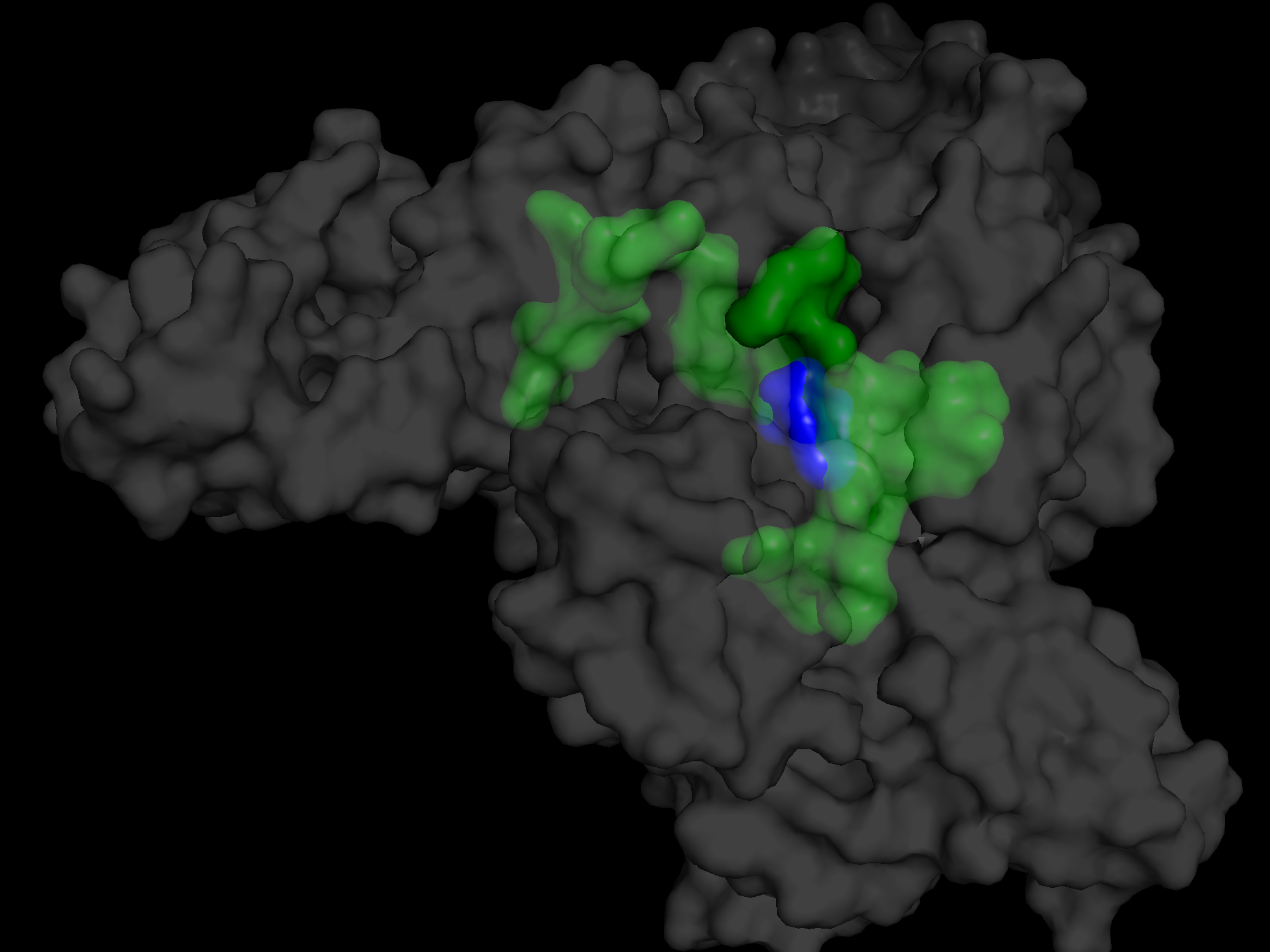 The transparent white/gray area is the protein.
The transparent green area is Pocket 1.
The blue area is the ligand, warfarin.
Summary:
We have shown how to use the tools, the basic work flow, and the meaning and importance of the stats given by the tools.
- Using PyMOL to visualize molecular structures.
- Using Open Babel to convert file formats (SDF to PDBQT).
- Using AutoDock Vina-GPU to perform molecular docking.
- Using conda to manage software environments.
- Using fPocket to find canidate location for docking.
Next we will cover more of the theory of how and why.